Universal Vehicle Traction Estimation Model: Comprehensive Research & Implementation

Executive Summary 

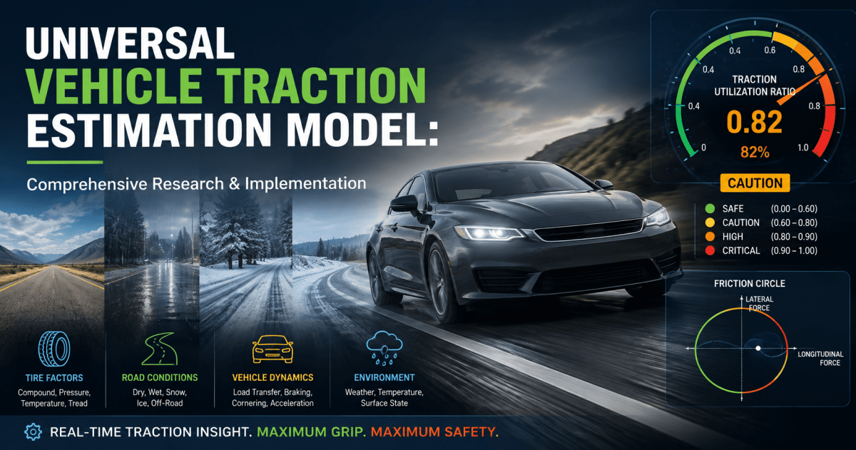
Traction is the tire’s grip on the road, fundamentally limited by friction between the tires and the surface. This comprehensive model provides a universal framework to estimate available traction capacity versus traction demand in real time, for any vehicle type (cars, trucks, EVs, etc.) and any road condition (dry/wet pavement, snow, ice, off-road). It combines well-established tire physics (e.g. Pacejka’s Magic Formula) with simpler fallback models (brush model, friction circle) to cover all scenarios. Every relevant independent variable is accounted for – from tire properties (compound, pressure, temperature, tread depth) and vehicle dynamics (load transfer during acceleration, braking, cornering) to environmental factors (surface type, weather). The model computes a Traction Utilization Ratio (TUR) – the fraction of available traction being used (0.0 to 1.0, or 0–100%). It also yields a Traction Safety Margin (remaining “grip headroom”) and categorizes current traction usage (safe, caution, critical) similar to an engine tachometer’s redline indicator. A default warning threshold (TUR ~0.80–0.85) triggers alerts to the driver when approaching the friction “redline.” The final deliverables include: 

• Step 1: Deep research on traction physics and factors influencing it, with references to authoritative sources. 

• Step 2: A full variable list (with default placeholders and units) covering tires, surface, vehicle, environment, and dynamic state parameters. 

• Step 3: Core mathematical equations for normal loads, friction limits (Magic Formula and friction ellipse), demanded forces, and computing TUR and safety margin. 

• Step 4: A robust, well-commented Python-like pseudocode function implementing the traction estimation logic, including default placeholders and calibration hooks for real-time use. 

• Step 5: Dashboard gauge design guidelines (tachometer-style traction meter with green/yellow/orange/red zones and digital readouts). 

• Step 6: Limitations (edge cases like hydroplaning, deep mud) and suggestions for validation and future improvements (integration with advanced sensors and ADAS). 

Together, these components enable a production-ready traction estimation system that is broadly applicable, self-contained, and easily visualized. 

[engineerfix.com], [racecar-en…eering.com], [suspension…rets.co.uk] 

Step 1 – Deep Research and Background 

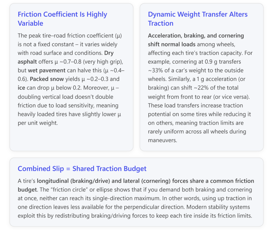
Traction and friction fundamentals: The maximum traction a tire can generate is governed by the laws of friction: the tire can only exert forces up to the product of the friction coefficient (μ) and its normal load (F). Classically, Coulomb friction posits *F = μ * F, but real tires deviate from this ideal. Tire friction is velocity-dependent, with distinct static and dynamic (sliding) friction; peak grip occurs at a small but nonzero slip ratio/angle, after which force falls off (“friction curve” or “grip slip curve”). For many tires, peak longitudinal friction occurs around 15–30% slip (i.e. wheel speed 15–30% different from free-rolling), while peak lateral friction occurs around ~6° of slip angle, beyond which sliding begins and force declines (the “friction cliff”). Kinetic friction (when the tire is sliding) is generally lower than peak static friction. The friction coefficient itself depends on myriad factors beyond just the two materials in contact. Road surface conditions (dry vs wet, tarmac vs gravel vs ice) drastically change μ. Tire rubber compound and tread also impact μ: for example, winter tires remain softer at low temperatures, improving grip on cold surfaces. Tire temperature influences friction via chemical and mechanical effects; warm tires usually grip better up to an optimal temperature, then degrade if overheated. Inflation pressure alters the contact patch size and shape, affecting grip – too low or too high pressure reduces contact area or effective adhesion. Tread depth helps channel water and bite into snow/mud; a worn tire (low tread) severely reduces wet and snow traction. [en.m.wikipedia.org] [racecar-en…eering.com] [engineerfix.com] 

Vehicle and weight distribution: The vehicle’s geometry and mass distribution set baseline normal loads on each tire and how they change with dynamic maneuvers. A typical car (≈1500 kg mass) with ~50% front weight distribution has static normal loads of ~0.5 mg on front vs rear axles. Load transfer occurs during acceleration, braking, or cornering: under straight-line braking, inertia shifts load to the front axle (forward pitch or “weight on nose”), increasing front F and reducing rear F. Under acceleration, load shifts rearward (rear squat). Approximately 22% of total weight shifts per 1 g of longitudinal acceleration for a typical car geometry (e.g. ~220 kg in a 1000 kg car at 1 g). Similarly, lateral acceleration causes roll and lateral load transfer: e.g., a 0.9 g turn with ~0.6 m CG height and 1.6 m track can shift ~33.7% of the car’s weight from the inside wheels to the outside wheels. These weight shifts directly alter each tire’s F, thus affecting each tire’s individual friction limit (since friction ≈ μ F). Moreover, vertical load sensitivity means μ itself is lower for heavily loaded tires – so distributing weight evenly (e.g. via low CG and balanced design) is advantageous for maximizing total grip. Suspension stiffness and anti-roll geometry also affect the fraction of load transfer taken by springs vs geometric load paths, influencing how quickly and how much weight shifts under transient maneuvers. [suspension…rets.co.uk] [racecar-en…eering.com] [vtechworks…lib.vt.edu] 

Combined-slip behavior: When a tire must concurrently produce longitudinal and lateral forces (e.g. braking while cornering), its total frictional capacity splits between these directions. The “friction circle” (or more accurately, friction ellipse) illustrates that the vector sum of lateral and longitudinal forces cannot exceed μF. In practice, combined-slip models (like Pacejka’s or friction ellipse) impose a limit: e.g., ( \sqrt{(F_x/(μF_z))^2 + (F_y/(μF_z))^2} \le 1 ). If one component (say braking force) is high, the other (cornering) must be lower to stay within the tire’s friction envelope. The Pacejka Magic Formula includes combined-slip extensions using weighting functions or normalized resultant slip to adjust the peak force when both slip ratio (κ) and slip angle (α) are nonzero. A simpler friction ellipse approach (also used in many control systems) scales down the available longitudinal force as lateral force increases (and vice versa), often assuming an elliptical coupling between the force components. [racecar-en…eering.com] [skill-lync.com] 

The Pacejka Magic Formula (MF): Developed by Hans Pacejka and colleagues, the Magic Formula is an empirical tire model that can accurately fit measured tire force curves over a wide range of slips. The general form expresses tire force Y (could be lateral F, longitudinal F, or aligning moment M) as: [skill-lync.com]