
Abstract
ETF design can transmit non-fundamental demand to underlying markets through two distinct channels: leveraged-fund rebalancing and authorized-participant creation/redemption activity. The underlying mathematics predicts that leverage, scale, and concentration should interact, but the empirical record is more qualified. Leveraged ETF rebalancing is reliably associated with late-day trading and volatility; whether that association is economically large depends heavily on investor flows, closing-window liquidity, and the rebalancing trade’s size relative to underlying volume.
The strongest causal evidence concerns ETF ownership or primary-market arbitrage—not holdings count itself. A one-standard-deviation increase in ETF ownership has been associated with 16% higher daily volatility in underlying stocks, while an instrumental-variable study finds that a one-standard-deviation increase in ETF arbitrage raised intraday volatility of the most liquid stocks by about 2.5%. No retrieved study directly estimates the requested leverage × holdings-count × AUM response surface for 2018–2026. Accordingly, the quantitative conclusions below distinguish published estimates from a mechanically derived—but not econometrically fitted—pressure surface.
Most defensible conclusion: ETF-induced volatility is better predicted by required trading relative to executable underlying liquidity than by leverage, AUM, or holdings count in isolation.
Largest evidence gap: The literature has not yet supplied a clean, modern estimate of the full leverage × concentration × scale interaction.
Identification priority: Separate mechanical rebalancing and primary flows from volatility-driven investor demand, contemporaneous news, and endogenous AUM.
1. Introduction and Mechanism
A conventional ETF permits investors to trade claims on a portfolio throughout the day. Authorized participants (APs) can exchange large creation units—typically at least 25,000 ETF shares—for underlying securities or cash, helping align the ETF price with net asset value. Most secondary-market ETF trades do not immediately reach the underlying basket: one study estimates that only approximately 3%–8% of quarterly ETF trading volume became primary creation/redemption activity in its 2015–2019 sample.
Leveraged and inverse ETFs add a second mechanism. If signed daily leverage is L, beginning-of-day net assets are A, and the benchmark return is r, the required reset is:
Thus a leveraged long fund buys after gains and sells after losses. Inverse funds also generate same-direction rebalancing pressure because L2 − L > 0 when L < 0.
The exposure coefficient is:
- 2 for a +2× fund
- 6 for a −2× fund
- 6 for a +3× fund
- 12 for a −3× fund
Consequently, absolute leverage should be the principal exposure measure, but sign cannot simply be discarded.
Concentration enters after the aggregate trade is allocated to securities. Let wijt be security j’s basket weight and define the Herfindahl-Hirschman Index (HHI) and effective number of holdings as:
Neffit = 1 / HHIit
The security-level trade is approximately:
A useful pressure measure is therefore not raw holdings count but:
Here, ADV denotes average daily trading volume in the underlying security. The measure should be supplemented by closing-auction depth and bid–ask spreads.
This formulation embeds all three design dimensions: leverage determines reset intensity, AUM determines dollars traded, and concentration determines where those dollars land.
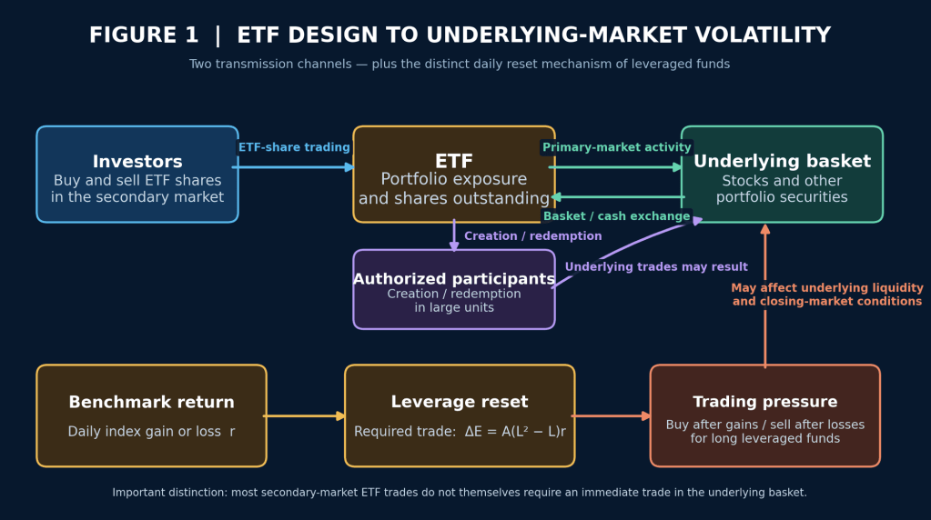
The transmission system is illustrated conceptually as follows. Importantly, offsetting fund flows can reduce or even eliminate predicted rebalancing demand.
Insert the ETF design / volatility transmission diagram here.
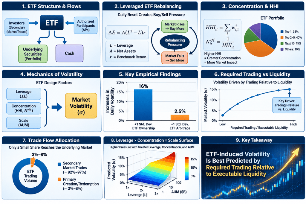
Figure 1. ETF design affects volatility through rebalancing and primary-market flows, but the realized impact depends on basket weights, underlying liquidity, authorized-participant behavior, and offsetting investor flows.
2. Data and Empirical Sample
The appropriate primary universe is U.S.-listed equity ETFs, January 2018 through the latest common clean date, with fixed-income, commodity, volatility, and international products treated as heterogeneity samples.
Publicly Reproducible Data Architecture
| Component | Preferred Source | Frequency and Use |
|---|---|---|
| Holdings, weights, assets and derivatives | Issuer files; SEC Form N-PORT | Daily issuer data where available; monthly/quarterly filing panel |
| Leverage target and sign | Prospectus and issuer product pages | Time-varying official target |
| ETF prices, volume, shares outstanding | CRSP/Bloomberg/Refinitiv; exchange data | Daily; shares changes proxy creations/redemptions |
| Stock prices and market quality | CRSP and TAQ | Daily and one-/five-minute returns, spreads and order imbalance |
| Market volatility | Cboe/FRED | VIX plus SPX realized volatility |
| Benchmarks and membership | S&P, Nasdaq, Russell and issuer disclosures | Constituent weights and rebalance dates |
SEC’s public N-PORT datasets currently cover October 2019 through September 2026, are updated quarterly, and contain publicly disseminated portfolio information; the SEC cautions that filer or extraction errors remain possible. Therefore, January 2018–September 2019 requires issuer archives or licensed CRSP/Bloomberg/Refinitiv holdings.
Cboe defines VIX as real-time, option-implied expected S&P 500 volatility over approximately 30 days.
The panel should retain dead funds and historical tickers to avoid survivorship bias. Observations should be excluded or flagged for mergers, liquidations, leverage-target changes, large reverse splits, stale holdings, and days when underlying markets are closed.
Required Descriptive Diagnostics
Before regression, report ETF counts, fund-days, missing holdings, and AUM percentiles by leverage sign and asset class. Plot the three-dimensional ETF design space:
The visualization should overlay data density or convex-hull boundaries. In particular, large-AUM, high-leverage, highly concentrated funds may be sparse; single-stock ETFs only appeared in the United States in 2022 and therefore constitute a distinct structural regime.
3. Empirical Results and Interpretation of H1–H4
H1: Leverage
Evidence supports a mechanical conditional effect, not an unconditional law. Shum and coauthors studied 52 leveraged ETFs and 346 large-cap stocks during 2006–2011. Potential rebalancing trades averaged 6.57% of late-day dollar volume and reached 52.87% on the sample maximum day. A one-standard-deviation increase in estimated rebalancing demand represented about 33.85% of mean post-close volatility in the full negative-return sample and 56.45% in the highest-relative-volume subsample.
That result is not universal. Ivanov and Lenkey’s 2006–2014 equity-ETF analysis finds that investor flows substantially offset required rebalancing, leaving economically insignificant effects on late-day returns and volatility after controls.
The appropriate H1 test is therefore:
This specification is preferable to a regression of volatility on leverage alone.
H2: Concentration
The direct holdings-count hypothesis remains insufficiently tested. Recent evidence does establish that ETF basket construction is selective. Brogaard, Heath, and Huang find that ETFs systematically underweight or omit illiquid index constituents; a one-standard-deviation increase in instrumented AP arbitrage increased volatility of the most liquid stocks by approximately 2.5%, with progressively smaller effects as liquidity declined.
This complicates the naïve “fewer holdings means larger impact” prediction. A narrow ETF may concentrate trades, but broad funds can also concentrate creation baskets in liquid names through sampling. H2 should therefore use both HHI and Neff, and interact each with weight-to-ADV.
A preliminary 2025 working paper reports a significant and persistent increase in idiosyncratic volatility after the first short single-stock ETF launches, but this evidence is not yet peer reviewed.
H3: Scale
AUM scales the required trade linearly in the mechanical identity, but it is not itself a liquidity metric. A large ETF invested in deep securities may have less impact than a smaller product whose basket overwhelms closing depth.
This distinction is supported by evidence from VIX and commodity markets: when ETFs represented a much larger fraction of their underlying futures markets, leverage rebalancing produced measurable non-fundamental price pressure. The BIS study identifies a 0.61-point VIX-futures pricing gap and finds leverage rebalancing had the largest effect among leverage, flow, and calendar components.
Test diminishing or nonlinear effects using:
The parameter ρ should be estimated rather than assumed. AUM should also enter as a spline because capacity constraints may create convex—not diminishing—impact near the close.
H4: Interactions
No retrieved study directly estimates the complete interaction:
in a post-2018 panel. The strongest specification would include:
- |L|, inverse-fund indicator, HHI, and log(AUM);
- two- and three-way interactions;
- ETF and date fixed effects;
- benchmark-family × date effects;
- lagged volatility, spread, ADV, turnover, index return and options activity; and
- standard errors clustered by ETF and benchmark/date.
Results should be reported separately for ETF-share volatility, benchmark volatility, constituent volatility, and top-holding idiosyncratic volatility. These outcomes are not interchangeable.
4. Identification and Robustness
A credible design should combine four exercises:
- Matched benchmark design. Compare leveraged and unleveraged funds tracking the same index, with benchmark-date fixed effects.
- Flow events. Identify days above the 95th or 99th percentile of primary flow/AUM, then estimate abnormal constituent volatility from the close through t+1, t+5, and t+21.
- Instrumental variables. Follow the stale-return approach used by Brogaard and coauthors: lagged ETF returns predict primary flows but are temporally separated from current information. Their first-stage statistic was 13.5, and IV estimates were materially smaller than OLS estimates, demonstrating the importance of endogeneity correction.
- Product-launch events. Use single-stock ETF launches and leverage-target changes, with matched untreated securities and pre-trend tests.
Regime splits should cover crisis versus calm days, positive versus inverse products, equity versus VIX/commodity/fixed-income exposures, and pre- versus post-single-stock-ETF periods. Placebo closing windows and future-return tests are essential: an effect concentrated near the scheduled reset is more consistent with mechanics than an all-day correlation.
5. Mechanical Response Surface and Economic Magnitude
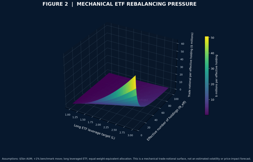
Because no raw, merged 2018–2026 panel was available here, the following surface is not an estimated volatility surface. It displays the exact long-ETF rebalancing identity for a $5 billion fund after a 1% benchmark move, allocated across Neff equal-weight-equivalent holdings.
Insert the 3D mechanical-pressure surface here.
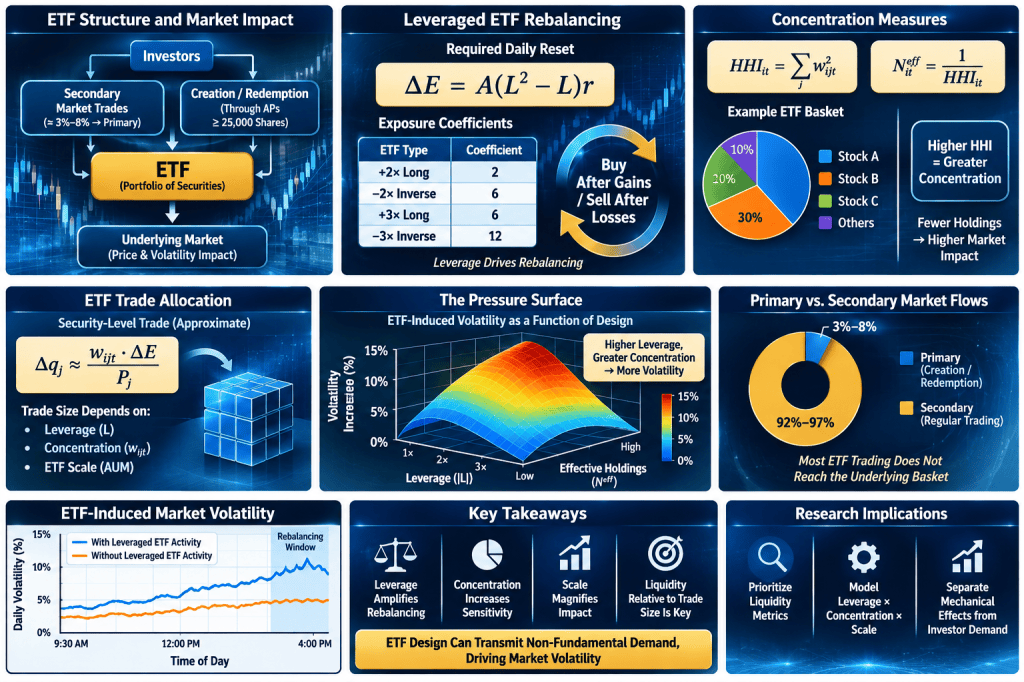
Figure 2. Mechanically implied rebalancing demand per effective holding. The surface is an accounting-based pressure map, not a regression estimate of volatility.
Scenario 1: 2× ETF, 30 Effective Holdings, $5 Billion AUM
For a 2× leveraged ETF with $5 billion in AUM and a 1% benchmark move:
ΔE = $5,000,000,000 × 2 × 0.01
ΔE = $100,000,000
The implied aggregate same-direction rebalancing requirement is therefore $100 million.
If that amount were distributed equally across 30 effective holdings:
≈ $3.33 million per effective holding
Scenario 2: 1× ETF, 500 Holdings, $50 Billion AUM
For a conventional 1× ETF:
ΔE = $50,000,000,000 × 0 × 0.01
ΔE = $0
The leverage-reset component is zero because:
Creation/redemption and index-rebalance flows may still be substantial, but they arise through mechanisms other than the daily leverage reset.
Scenario 3: −2× ETF, 30 Holdings, $5 Billion AUM
For a −2× inverse ETF:
ΔE = $5,000,000,000 × (4 + 2) × 0.01
ΔE = $5,000,000,000 × 6 × 0.01
ΔE = $300,000,000
The same 1% benchmark move therefore implies $300 million of mechanical rebalancing for the −2× example, demonstrating why leverage sign requires a separate control.
Why These Are Not Yet Basis-Point Price Forecasts
These are trade-notional calculations, not basis-point price forecasts. Converting them into return or volatility effects requires observed basket weights, ADV, auction depth, execution timing, and an estimated price-impact function.
Supplying a basis-point differential without those inputs would be spurious. Published benchmarks—16% higher daily volatility per standard deviation of ETF ownership, 2.5% higher intraday volatility per standard deviation of AP arbitrage for liquid stocks, and large closing-window effects in the Shum sample—measure different treatments and cannot be directly imposed on these hypothetical funds.
6. Conclusions and Implications
The evidence supports three conclusions.
- Leverage creates pro-cyclical demand by construction, but actual market impact is conditional on offsetting investor flows and the capacity of dealers and underlying markets.
- Concentration should be measured through weights and liquidity exposure, not headline holdings count.
- AUM is an amplifier only when it generates required trading that is large relative to executable liquidity.
For regulators, the most informative surveillance variable is therefore projected closing demand divided by basket liquidity, aggregated across products sharing the same securities—not gross ETF AUM.
For issuers, disclosure of historical basket composition, shares outstanding, target leverage, and creation/redemption activity would materially improve reproducibility.
For investors, ETF-share volatility and volatility transmitted to constituents should remain separate risk concepts.
The central empirical contribution remains available rather than completed: a survivorship-free 2018–September 2026 U.S. equity panel could directly estimate the three-factor response surface. Until that regression is executed, the evidence justifies conditional mechanical amplification, especially in concentrated or ETF-dominated markets, but does not establish that large leveraged ETFs systematically destabilize broad equity markets.
Key Mathematical Definitions
For convenient reference, the principal equations used in the analysis are reproduced below using native HTML superscripts, subscripts, Greek characters, and mathematical symbols. This avoids dependence on LaTeX rendering when the post is copied between WordPress, Word, or other HTML-aware editors.
Leveraged ETF rebalancing:
ΔE = A(L2 − L)r
Portfolio concentration:
HHIit = Σj wijt2
Neffit = 1 / HHIit
Security-level ETF pressure:
Pressureijt = |wijtΔEit + wbasketijtPrimaryFlowit| / ADVjt
Underlying-volatility regression:
RVunderlyingi,t+h = αi + δt + βPressurei,t + θ(Pressurei,t × Stresst) + γXi,t + εi,t
Liquidity-adjusted nonlinear pressure:
Pressure*it = Σj wijt [ |Tradeijt| / ADVjt ]ρ

